In 2016, I published a paper on perception of differences between standard resolution audio (typically 16 bit, 44.1 kHz) and high resolution audio formats (like 24 bit, 96 kHz). It was a meta-analysis, looking at all previous studies, and showed strong evidence that this difference can be perceived. It also did not find evidence that this difference was due to high bit depth, distortions in the equipment, or golden ears of some participants.
The paper generated a lot of discussion, some good and some bad. One argument presented many times as to why its overall conclusion must be wrong (its implied here, here and here, for instance) basically goes like this;
We can’t hear above 20 kHz. The sampling theorem says that we need to sample at twice the bandwidth to fully recover the signal. So a bit beyond 40 kHz should be fully sufficient to render audio with no perceptible difference from the original signal.
But one should be very careful when making claims regarding the sampling theorem. It states that all information in a bandlimited signal is completely represented by sampling at twice the bandwidth (the Nyquist rate). It further implies that the continuous time bandlimited signal can be perfectly reconstructed by this sampled signal.
For that to mean that there is no audible difference between 44.1 kHz (or 48 kHz) sampling and much higher sample rate formats (leaving aside reproduction equipment), there are a few important assumptions;
- Perfect brickwall filter to bandlimit the signal
- Perfect reconstruction filter to recover the bandlimited signal
- No audible difference whatsoever between the original full bandwidth signal and the bandlimited 48 kHz signal.
The first two are generally not true in practice, especially with lower sample rates. Though we can get very good performance by oversampling in the analog to digital and digital to analog converters, but they are not perfect. There may still be some minute pass-band ripple or some very low amplitude signal outside the pass-band, resulting in aliasing. But many modern high quality A/D and D/A converters and some sample rate converters are high performance, so their impact may be small.
But the third assumption is an open question and could make a big difference. The problem arises from another very important theorem, the uncertainty principle. Though first derived by Heisenberg for quantum mechanics, Gabor showed that it exists as a purely mathematical concept. The more localised a signal is in frequency, the less localised it is in time. For instance, a pure impulse (localised in time) has content over all frequencies. Bandlimiting this impulse spreads the signal in time.
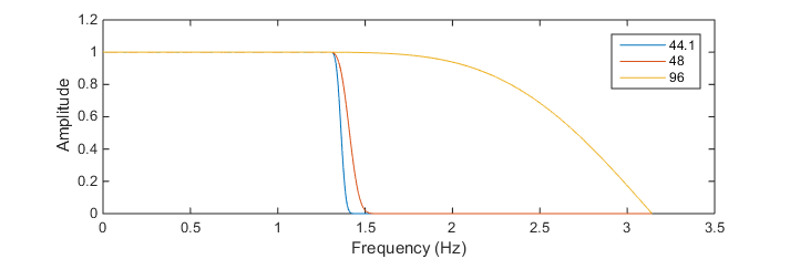
For instance, consider filtering an impulse to retain only frequency content below 20 kHz. We will use the matlab function IFIR (Interpolated FIR filter), which is a high performance design. We aim for low passband ripple (<0.01 dB) up to 20 kHz and 120 dB stopband attenuation starting at 22.05, 24, or 48 kHz, corresponding to 44.1 kHz, 48 kHz or 96 kHz sample rates. You can see excellent behaviour in the magnitude response below.
The impulse response also looks good, but now the original impulse has become smeared in time. This is an inevitable consequence of the uncertainty principle.

Still, on the surface this may not be so problematic. But we perceive loudness on a logarithmic scale. So have a look at this impulse response on a decibel scale.

The 44.1 and 48 kHz filters spread energy over 1 msec or more, but the 96 kHz filter keeps most energy within 100 microseconds. And this is a particularly good filter, without considering quantization effects or the additional reconstruction (anti-imaging) filter required for analog output. Note also that all of this frequency content has already been bandlimited, so its almost entirely below 20 kHz.
One millisecond still isn’t very much. However, this lack of high frequency content has affected the temporal fine structure of the signal, and we know a lot less about how we perceive temporal information than how we perceive frequency content. This is where psychoacoustic studies in the field of auditory neuroscience come into play. They’ve approached temporal resolution from very different perspectives. Abel found that we can distinguish temporal gaps in sound of only 0.4 ms, and Wiegrebe’s study suggested a resolution of 0.72 ms. Studies by Wiegrebe (same paper), Lotze and Aiba all suggested that we can distinguish between a single click and a closely spaced pair of clicks when the gap between the pair of clicks is below one millisecond. And a study by Henning suggested that we can distinguish the ordering of a high amplitude and low amplitude click when the spacing between them is only about one fifth of a millisecond.
All of these studies should be taken with a grain of salt. Some are quite old, and its possible there may have been issues with the audio set-up. Furthermore, they aren’t directly testing the audibility of anti-alias filters. But its clear that they indicate that the time domain spread of energy in transient sounds due to filtering might be audible.
Big questions still remain. In the ideal scenario, the only thing missing after bandlimiting a signal is the high frequency content, which we shouldn’t be able to hear. So what really is going on?
By the way, I recommend reading Shannon’s original papers on the sampling theorem and other subjects. They’re very good and a joy to read. Shannon was a fascinating character. I read his Collected Papers, and off the top of my head, it included inventing the rocket powered Frisbee, the gasoline powered pogo stick, a calculator that worked using roman numerals (wonderfully named THROBAC, for Thrifty Roman numerical BACkward looking computer), and discovering the fundamental equation of juggling. He also built a robot mouse to compete against real mice, inspired by classic psychology experiments where a mouse was made to find its way out of a maze.
Nyquist’s papers aren’t so easy though, and feel a bit dated.
- S. M. Abel, “Discrimination of temporal gaps,” Journal of the Acoustical Society of America, vol. 52, 1972.
- E. Aiba, M. Tsuzaki, S. Tanaka, and M. Unoki, “Judgment of perceptual synchrony between two pulses and verification of its relation to cochlear delay by an auditory model,” Japanese Psychological Research, vol. 50, 2008.
- Gabor, D (1946). Theory of communication. Journal of the Institute of Electrical Engineering 93, 429–457
- G. B. Henning and H. Gaskell, “Monaural phase sensitivity with Ronken’s paradigm,” Journal of the Acoustical Society of America, vol. 70, 1981.
- M. Lotze, M. Wittmann, N. von Steinbüchel, E. Pöppel, and T. Roenneberg, “Daily rhythm of temporal resolution in the auditory system,” Cortex, vol. 35, 1999.
- Nyquist, H. (April 1928). “Certain topics in telegraph transmission theory“. Trans. AIEE. 47: 617–644.
- J. D. Reiss, ‘A meta-analysis of high resolution audio perceptual evaluation,’ Journal of the Audio Engineering Society, vol. 64 (6), June 2016.
- Shannon, Claude E. (January 1949). “Communication in the presence of noise“. Proceedings of the Institute of Radio Engineers. 37 (1): 10–21
- L. Wiegrebe and K. Krumbholz, “Temporal resolution and temporal masking properties of transient stimuli: Data and an auditory model,” J. Acoust. Soc. Am., vol. 105, pp. 2746-2756, 1999.
